Last year I joined Gartner’s Supply Chain Executive Conference in London. I attended a presentation by Tim Payne, a Gartner Research VP focused on Supply Chain Planning. The presentation title was “A Strategic Road Map for Supply Chain Technology”. One of the key questions for someone interested in acquiring supply chain technology is of course where the biggest opportunity for improvement lies.
In a 2014 Gartner survey respondents were asked to indicate the top 3 obstacles to achieving their organization’s supply chain goals and objectives. The number one obstacle indicated was “Forecast Accuracy and Demand Variability.”
This is a theme we have given a lot of thought and attention to lately. In this post, I’d like to elaborate a bit about forecast accuracy and demand variability and introduce a recent innovation in this area, now part of our latest release IFS Applications 9.
Forecast Accuracy is an estimate of the quality of the forecast. Often people tend to see the forecast as an absolute number; you may hear that the forecast for Q1 is 1,000 units, but rather than an absolute number a forecast is a distribution of probability. How certain or uncertain the forecast is can be indicated by an estimate of the Forecast Accuracy expressed, for example, as Predicted Forecast Error.
In order to understand forecast accuracy we must measure forecast error. There are many ways to do this.
One example is our module for statistical forecasting, IFS Demand Planning. For each forecast flow (for example, product and delivery location), the system will calculate Mean Average Percentage Error, Mean Average Error and Mean Squared Error to mention a couple of the indicators available. What they all have in common is that they indicate the difference between the forecast and the actual results historically.
Does this now mean that the forecast error tells us how good or bad a forecast is? It actually would, if all products were equally difficult to forecast. But since this is never the case, looking at the forecast error alone is not a reliable indication of the quality of the forecast. We need one more variable to the equation, volatility.
Volatility is a way of expressing the variation in demand between periods. The variability can be divided into two parts:
- Stochastic variability
- Predictable variability. Known factors such as seasonality and campaigns will cause demand to change, but in a predictable way.
Good forecasting techniques and processes will decrease the forecast error caused by predictable variability. This is achieved by using, for example, seasonal profiles or forecasting models including trend components.
Stochastic variability, on the other hand, is caused by random events out of the forecaster’s control. If the stochastic variability is large, the forecast error will inevitably increase. And vice versa: the error will decrease for stable demand.
This is by no means an indicator of how successful the forecasting process really is.
Instead we need a holistic approach and analyze the forecast error together with the demand variability that caused it. A matrix like the one below can serve to explain this concept.
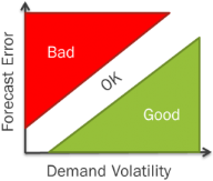
Low volatility, yet high forecast error indicates a bad forecast and that something should be done. High volatility and low error on the other hand indicates a good forecast.
Based on this approach we now have a way to determine the forecast quality in a comparable way defined as the quote between the forecast error and the demand volatility.
We have established a model to decide if forecasts are good or bad. The next question is to which extent these better or worse forecasts actually benefit or harm the business? Supply chain success is measured as customer service and cost. Good forecasts are fundamental to achieve high service levels and inventory turns.
The question is often which products to focus on first, where should planners make an extra effort to improve the forecasts?
One way of highlighting this is to look at the value of the forecast error. A systematic approach to improve the forecast for those products with the largest error value first will yield the most out of such an initiative.
As I mentioned earlier, IFS recently released IFS Applications 9. One of the new elements in the Demand Planning solution is a graph shown below:

Forecast Error Analysis Graph, IFS Applications 9
This new graph works exactly as outlined above. Based on a selection, for example a product group or a market the graph will plot all products. It is easy to find products with large errors and jump directly from here to the forecast graph to look at ways to potentially improve the forecast.
Maybe the forecast model is too slow, maybe it is a new product and the initial forecast turned out to be wrong, etc. Once the forecast has been fixed the product can be easily filtered from the graph in order to support a continuous effort to improve those forecasts that matters the most to the business.
Gartner’s research indicate that issues related to forecast accuracy and demand variability is on top of many companies’ agendas for supply chain improvement. With the structured approach to attack issues related to forecast accuracy and demand variability now available in IFS Demand Planning, we hope to help many of our customers with their number one obstacle on their path to supply chain improvement.
- For detailed information about IFS Applications 9 and what it can do for you, please download the brochure.